Scientific Computing

KPG-49D may not work from WINE. If not, boot into Windows or use a Windows virtual machine for programming Version 2 Kenwood 900MHz radio.

Note: A yellow exclamation point over the USB to serial adapter in Device Manager may indicate an obsolete version of the Prolific 2303. You can either replace the cable or use older Windows version.

This procedure is for VERSION 2 radios only! Version 1 uses the DOS software KPG-35D.

Install KPG-49D and then install the ham utilities:

KW900EZP_WIN7.zip
KWX81ETA_WIN7.zip
KwID.zip

To connect to the Beaglebone Black via SSH, use a USB to FTDI converter to J1. Be sure not to connect the Vdd, 5V, 3.3V or any pin providing voltage to J1!

Beaglebone Black J1 pinout:

There is no standard pinout for the USB to FTDI adapters, but the pins are normally labeled on the USB to FTDI adapter board.

1. connect the USB to FTDI adapter to the Beaglebone Black (you might use a USB extension cable–I’ve had good luck over the years with the Keyspan USA-19HS)
2. open up PuTTY and set the baud rate to 115200 8-N-1 and the COM port to match Device Manager in Windows or terminal.
3. Hit Enter a couple times on your laptop and you should see the login prompt.

The danger of cheap non-temperature regulated soldering irons is that the cheap soldering irons go from too hot when starting to solder the joint to too cold from cheap tip materials with poor thermal conductivity. This leads to joints that have cavities and are improperly flowed, especially a problem for radio frequency or high speed digital circuits. Cheap soldering irons lead the newbie or even the experienced user to burn parts, lift PCB traces off the board and get so hot they are very uncomfortable to hold. Often the cheap irons are not grounded, so you could be zapping the circuit you’re trying to fix.

For the beginner, there are $40 soldering stations available from reputable online sources–checkout the reviews or YouTube to get a better sense. For me as a life-long electronics guy, I went straight to Weller (Hakko is good, too). I strongly recommend the Weller WES51 temperature controlled soldering iron for those who outgrow the use of the local maker-space or borrowing a friend’s iron. I emphasize the temperature controlled part because even the Weller WLC100 does not have closed-loop temperature control.

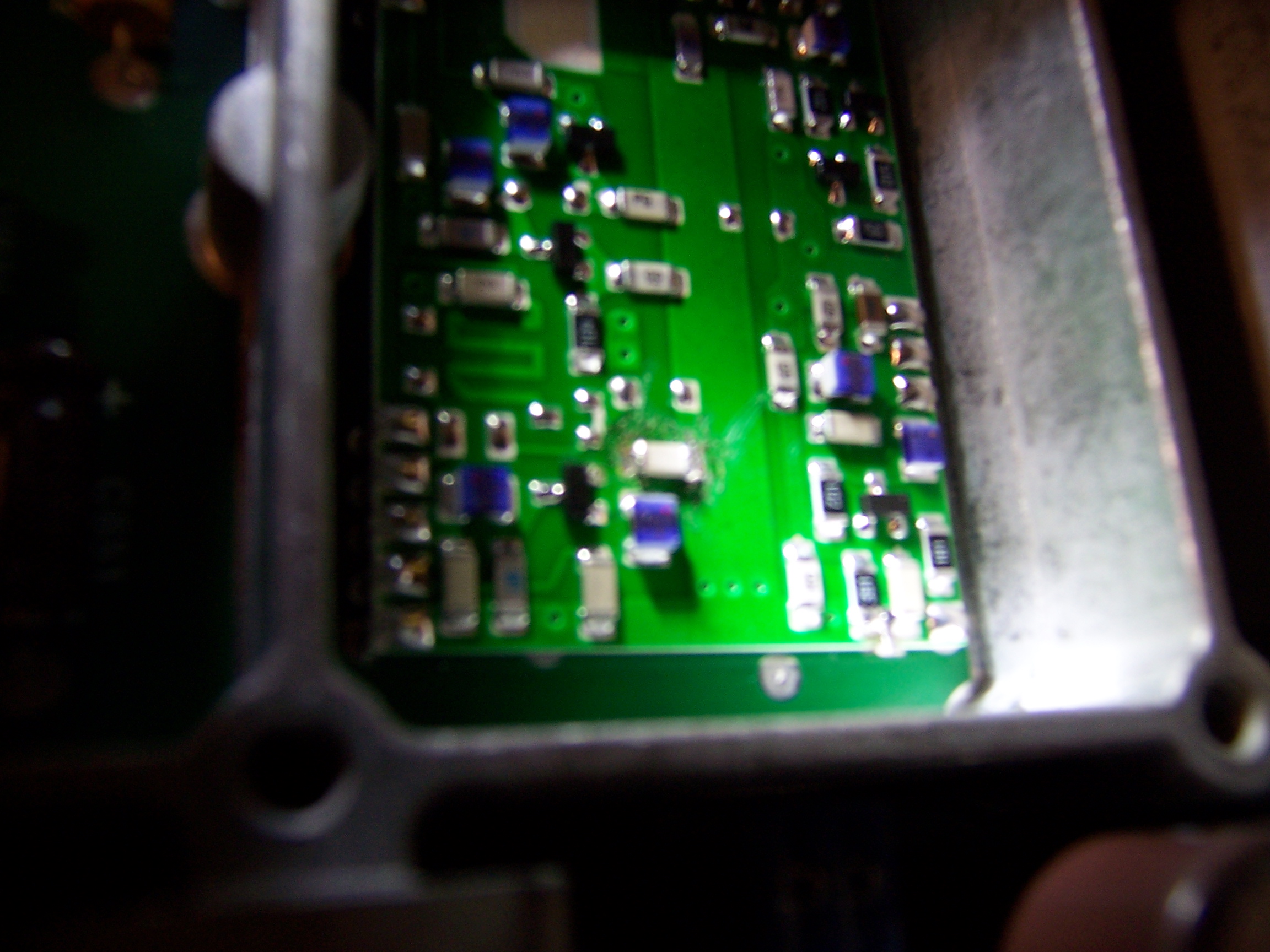
Many things we solder these days are of small size and delicate, so you don’t want to just guess at the temperature you’re using. The Weller WES51 is rated at maintaining the tip +/- 6 degrees Celsius from the setting. The WES51 has an analog temperature dial, which is close enough even with surface mount components, as you see in the photo below. It’s hard to see due to the focus, but the new white cap at the center of the picture soldered in like a dream, using the optional 1/32" tip.

For about 50% more cost you get the digital temperature readout Weller WESD51. We prefer the analog WES51 because one can change the temperature setting more quickly on the WES51 (just spin a dial vs. push and hold button on the WESD51), and it’s not necessary to have a perfect temperature setting or to lock the setting (perhaps something a factory assembly line would do).

25 JUNE 2015 CEDAR workshop presentation on using Astrometry.net algorithm to register image with stars.

Jeff Cogswell’s article Learning Enough Python to Land a Job. calls out that Python is for more than web development, Django, Twisted, Flask, &c. As a data science practitioner, mangling tens of gigabytes if not tens of terabytes daily from sensors deployed around the globe, converting code to Python after several years of hard-core Matlab use was motivated by Python’s highly-performant data science stack incorporating Pandas, SciPy, Numpy, h5py and other specialty Python user modules.

1. Port code gradually, even from very high-level languages like Matlab. Tools like f2py for Fortran 77/90+, SWIG (and numerous others) for C, Oct2Py for Matlab, etc. allow you to speedily and often straightforwardly integrate code from other popular languages.
2. Get familiar with (in this order): Spyder, Numpy, Matplotlib, h5py, Scipy, and Pandas. If you’re working with most real problems, you should be considering Pandas and h5py to allow you to filter/select data before reading it all form disk. I personally prefer h5py over PyTables. The fastest data to load is data where the superfluous data you didn’t need was never loaded, that would otherwise slow down the loading of the wanted data!
3. Get started in data analysis knowing not much more than how to use dict(), list(), and numpy.array() along with the standard basic functions that one would use in Matlab or R. such as sqrt(), for, if, &c. Learn about Numpy and Pandas before dealing with generators, sets, list comprehensions, itertools, etc.
4. When you find you have lots of heterogeneous but associated variables, particularly those associated by time, it’s time to use Pandas. Beyond 2-D DataFrames, xarray is the module to use. Pandas is awesome for loading and working with large heterogenous datasets. Think of Pandas as SQL for doing computations.

We hope this commentary on Python for data scientists and analysts considering the transition to Python from languages such as R, Matlab, Fortran, etc. has helped you.

To overlay a contour on top of a Matlab “image()” or “pcolor()”, first rasterize the image and then overlay a contour to make it work in a 3-D Matlab figure. This is a bit complex to describe, so we created an example of contour over image in a 3-D Matlab figure: contourImage2.m. This script follows these steps:

1. flatten the contour onto the image in the default z=0 plane
2. render as a resized image
3. make a pcolor plot
4. manipulate the underlying Surface object to an arbitrary 3-D location.

Doing a contour overlay on a 2-D image or pcolor is much simpler especially in Python.

Matlab does not require special manipulations via freezeColors of the figure colormap in order to have a unique colormap for each axes (subplot) on a figure. examples

Brilliant Hackaday SDR radar article by  Juha Vierinen

Uses $8 USB RTL-SDR sticks and cheap antennas to detect reflections from airplanes, the ionosphere, and more!

If the man command on Linux isn’t working, check that the manual database is installed:

apt install man-db

matplotlib.ticker.ScalarFormatter configures the colorbar and axes labels to not have too many decimal places.

ScalarFormatter Problem

If I made a standard line plot using the ScalarFormatter passed into a function, then subsequently passed the ScalarFormatter into another function that used colorbar, the line plot y-axis would be reset to match the limits of the later figure’s colorbar.

I didn’t think the ScalarFormatter would be able to feedback like that.

Fix ScalarFormatter

Enclose ScalarFormatter in its own function, then call that function from each of the plotting functions, thereby creating a new/unique ScalarFormatter for each figure.