FMCW GNU Radio such as
FMCW_usrp.grc
setup is common to several IEEE articles.
Do these setups actually work as shown?
This general process is used for the PiRadar Red Pitaya
radar code.
The method extends to any short range radar using CW or FMCW modulation.
The signal processing algorithm must read/process the data in small segments.
This is the only way to make a real time measurement.
It conserves RAM/CPU for offline analysis as well.
Verify the data is read correctly–the raw data must make sense when plotted, or nothing else will work.
Many software defined radios output complex single-precision floating point data.
Often this data consists of 4 byte pairs of real/imaginary coefficients.
Matlab can read such data with Matlab script for complex data
as in read_complex_binary.m.
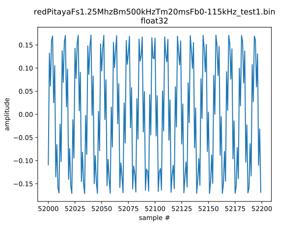
Incorrectly read FMCW sinusoid data--note very distorted waveform is NOT read correctly.
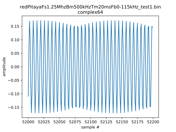
Correctly read FMCW sinusoid data--note clean sinusoid waveform, with at least two closely frequency-spaced sinusoids.
Slice FMCA data by chirp for processing.
FMCW data and radar data in general is arranged into segments for each radar pulse/chirp so that you can estimate the covariance across FMCW chirps.
This can be done by inspection since we’re only using a couple files to start.
The chirp spacing is regular in number of samples–same throughout the entire file.
For example, if the radar pulses at 10 Hz –> every 100 ms is a new measurement.
When you’ve put these into a 2-D array, plot the data again to see the data is sliced correctly.
The 2-D array has each pulse/chirp data in a row, and the columns are sample number.
Thus if I analyze 8 chirps each of 1024 samples, the array has shape 8 x 1024.
Estimate FMCW beat frequencies to get range.
For FMCW radar, where the frequency sweep is linear, if target A gives a 1 Hz sinusoid and target B gives a 2 Hz sinusoid, target B is twice as far away as target A.
Measuring absolute range starts with determining what zero range is in beat frequency.
Just like real targets, the zero range (feedthrough) of the radar (which is the radar hearing its own transmission) shows up as a sinusoid.
In general the radar hears itself as the lowest frequency sinusoid and also at the largest amplitude.
In a synchronized radar, this zero range feedthrough frequency (let’s call it F0) is constant for a particular radar configuration.
F0 changes for each unique radar configuration (antennas, RF channel used, RF bandwidth used, etc.).
In an unsynchronized radar such as the Red Pitaya currently is, F0 might change each time the same program is run, or even occasionally while the program is running.
However the same problem occurs whether synchronized or unsynchronized (or measuring a jet engine)–one must first find F0.
We measured with one of the Red Pitaya in FMCW radar mode that F0 stays constant for at least ~10 seconds at a time
Because F0 is so much larger in amplitude than any other sinusoid, you can do this with classic DFT (implemented via FFT) methods.
These methods will find F0 approximately, with a few percent error.
You will find F0 accurately with subspace estimation later.
To make the frequency estimation problem not consume an extremely large amount of RAM and CPU, we first reduce the problem as follows.
If F0 is 100 kHz, but the maximum target frequency is 10 Hz, that is, we know that the only frequencies we’ll ever use are between 100,000-100,010 Hz, the problem because much easier to process if we first:
frequency translate – multiply by complex sinusoid, this rotates the discrete-time samples in frequency, analogous to a shift register
downsample – by anti-alias filtering and decimation e.g. scipy.signal.decimate()
Thus instead of working with a file sampled at 4 MHz, we can downsample to 8 kHz, which conveniently you can play through your PC sound card if you want.
When the target is not present, you hear a single tone, the F0 of the radar, plus low amplitude clutter.
FMCW software defined radar processing: CWsubspace.py.
When the target is introduced near to the radar antenna, say 1-2 meters away, held still, not moving, you hear the F0 sinusoid apparently wavering in amplitude as that’s how closely frequency-spaced sinusoids behave–the amplitude envelope rapidly grows and shrinks for a tremolo effect like on the musical organs used at baseball games.
FFT-based methods exhaust RAM and CPU long before one can solve closely spaced sinusoid frequency estimation problems.
The family of subspace frequency estimation techniques include RootMUSIC and ESPRIT, implemented in
Python.
These Python subspace estimation functions such as ESPRIT are also callable from
Matlab.
These functions output estimated frequencies and the singular value sigma, which can be taken as a confidence measure of the estimate.
Informally, σ < 1 indicates low confidence–this estimate is suspect.
σ ≫ 1 indicates a high confidence, values in the tens or hundreds are possible in high SNR data.
Convert FMCW beat frequency to range using sigma as a qualifier, and that F0 is the lowest frequency, we convert target FMCW beat frequencies F_t to range R_t by:
R_t [meters] = c * F_t * T_m / (2*B)
Where c is speed of light, T_m is PRI i.e. time to sweep up or down in frequency, and B is the sweep bandwidth [Hz].
In general an FMCW radar measures F_t as F_t,measured = F_t,true + F0.
Unlike analog FMCW radars, software-defined radars must typically have a broad enough bandwidth to catch the entire chirp bandwidth.
Unless for example one used an external VCO and the SDR can readily accept such, typical Ettus SDRs cannot quickly and deterministically change center frequency.
At that point, you have simply a system more like the hardware-based radars, since you would be restricted to FMCW mode only for broad bandwidth.
Instead, it is more desirable in general to have enough ADC/DAC bandwidth so that a chirp is synthesized within the ADC/DAC bandwidth and sent/received with SDR hardware VCO at a constant frequency.
With today’s SDRs, that limits chirp bandwidth to the 1-100 MHz range, maybe order 1 GHz with a high-end SDR.
The FPGA or CPU has to be powerful enough to handle this streaming data rate–with a moderate PC and Ettus B200, you might get 5 MHz chirp bandwidth because you have to account for USB congestion and CPU utilization based on total TX + RX bandwidth.
Of course, with RFNoC (if your SDR supports RFNoC) you can benefit greatly from processing directly on the FPGA.
Assuming the network/connection between the PC and SDR is stable, there should be a constant offset in number of samples between transmit and receive for a given radar configuration (e.g. sample rate, etc.).
Factors contributing to instability in terms of number of samples offset include: using virtual machine instead of directly running operating system, Wifi, congested Ethernet network, etc.
gr-radar has an approach to working around these issues by assuming the offset is at least constant for a particular run.
gr-radar computes the sample offsets for a run.
However, this OOT GNU Radio module is more oriented toward UHD Open Source driver, which is for Ettus Research SDR and other SDRs including Per Vices, Cubic SDR.
The Red Pitaya does not yet appear to implement UHD, but rather uses its own method of transferring streaming data PC ↔ hardware.
GNU Radio is oriented around streaming signals.
In many forms of radar, one is oriented around pulsed signals.
That is, one could get around the synchronization issues of streaming signals by getting the transmitter and receive cued up, and then starting both RX/TX together with deterministic FPGA delay.
For many interesting radar systems there is more than one radar within range of targets and each other, so that a form of multiplexing channel access is necessary.
For FMCW, TDMA and FDMA are two popular radar multiplexing methods.
For embedded radar system networks, where running on solar power, or where using small economical CPUs, streaming processing may be beyond the needs and/or budget.
This leads one to a non-GNU Radio pathway, as Pavel has been exploring with a number of Red Pitaya configurations.
Specifically, Pavel has provided a prototype radar Red Pitaya SD card
image
setup, such that individual pulses can be sent with the receive and transmitter synchronized.
GNU Radio gr-radar added the “Echotimer” self-calibration function in 2014.
Workaround these issues for non-USRP radars as mentioned in the first section.
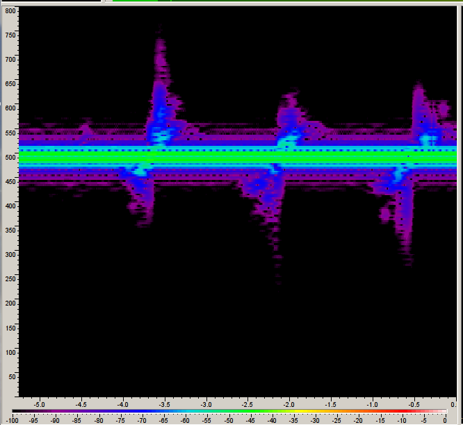
Spectrogram of 1 m/s moving target with USRP at 5.75 GHz, sweeping 1 MHz. Horizontal axis is time in seconds, vertical axis is frequency in Hz.
The moving 30x40 cm tinfoil piece was moved up and down from almost touching the radar antenna to about 1 m away.
The main frequency displacement from the radar feedthrough was due to the Doppler shift.
To reduce the signal processing burden, one can sweep over say 10 MHz if possible as this increases the tone separation.
The main point is to show that the USRP with plain GNU Radio FMCW was stable, even when restarting the program.
This spectrogram was created by:
Ettus B200 with 5 cm piece of wire stuck in each of the TX/RX and RX2 ports for antennas
FMCW_usrp.grc sweeps from 5.750 GHz to 5.751 GHz, recording a 4Mbps complex float32 stream to disk of the beat frequencies. However, we know the beat frequencies will be very closely spaced (< 1 kHz) from feedthrough. This could be combined with next step if CPU can handle it. Obviously this would ideally be done on the FPGA.
PlaybackFMCW.grc filters and downsamples about the feedthrough frequency, where a 16 kbps complex64 stream is more than enough for any possible beat frequencies. It writes a .wav file for convenience.
FMCW_load_process_data.py takes the .wav file, windows it, chopping out the bad interpulse data.
Using Goldwave or Audacity, listen to the wave file and get the live spectrogram.
MATLAB on Linux claims to only playback uncompressed AVI files on “UNIX” systems.
However, MATLAB on Linux can’t even play all uncompressed AVI filed depending on your particular system configuration with gstreamer.
A workaround for MATLAB codecs is using Motion JPEG in AVI videos by converting the video with
FFmpeg:
thread[thread-per-block[3]: <block gr uhd usrp source (1)>]: EnvironmentError: IOError: Radio ctrl (0) packet parse error - AssertionError: packet_info.packet_count == (seq_to_ack & 0xfff)
  in uint64_t radio_ctrl_core_3000_impl::wait_for_ack(bool)
  at /build/uhd-fDtHan/uhd-3.9.2/host/lib/usrp/cores/radio_ctrl_core_3000.cpp:264
This error can indicate there is an excessive dataflow rate.
Try reducing your sample rate.
Check if you’re connected via USB 3 and not USB 2 (is USB Type A all the way into the computer USB 3 jack?) Check via:
dmesg
You should see
new SuperSpeed USB device number 3 using xhci_hcd
LPM exit latency is zeroed, disabling LPM.
New USB device found, idVendor=2500, idProduct=0020
New USB device strings: Mfr=1, Product=2, SerialNumber=3
Product: USRP B200
Manufacturer: Ettus Research LLC
This post documents the procedure from acquiring noisy, distorted CW radar data through drawing conclusions for the next steps in Red Pitaya radar development.
Read the data into the computer memory appropriately.
GNU Radio complex is single-precision float, marshaled as real/imag pairs of 4 byte floats.
Matlab: read GNU Radio complex data with read_complex_binary.m that reshapes and casts the data appropriately.
Python: numpy.fromfile(filename,'complex64')
An example command from the piradar program is
./PlotSpectrum.py exercise.bin 100e3
where we see the 60 Hz periodic interference, which we model in the next section.
If the sinusoids are not clearly and cleanly present, or the audio playback doesn’t sound like a pure sinusoid, something is very wrong–stop at this point and fix the problem.
Signal defects may come from software and/or hardware.
They may have subtle or visible effects.
An empirical model was created based on the appearance of ADC clipping in the time and frequency domain in the piradar program SimADCclipping.py
./SimADCclipping.py
This model gives the basis to build filters suitable for preprocessing before using subspace estimation of close-spaced CW sinusoids typical to CW radar with Red Pitaya or any other such instrument.
Without filtering, the subspace estimator homes in on the forest of 60 Hz “fake” targets.
One can create remarkable filters in the simulation or analytic space.
Whether they can be realized in a real system depends on the CPU/FPGA power available in the real system and if they require excessively precise frequency/phase control and the like.
Here’s let’s assume we can use a FIR filter with order 4096 taps to reduce signals greater than +/- 60 Hz from the CW radar center frequency by about 20 dB and much more reduction beyond that.
The center frequency chosen is for a radar baseband center frequency of 10 kHz.
The text file cwfir.asc contains FIR filter coefficients used in the next step.
FIR filters are used in perhaps the vast majority of electronic devices.
In contrast with IIR filters, which are generally realized with far fewer taps (less computational effort) for a given specification, FIR filters have linear phase in-band, while IIR filters in general do not.
The signal_subspace program has both a Python and Fortran implementation of a FIR filter.
However, there is also a filter built into scipy.signal.decimate.
This offline analysis used SciPy’s filter.
After downconversion, the signals look like the following, with and without target.
How much to downconvert is driven by the signal bandwidth.
Downconversion will act like a shift register for the analytic signal in frequency.
Downconverting the signal might take place most effectively in multiple steps if extreme ratios are involved, such as might occur in software defined radar.
This is where RFNoC or custom FPGA programming can conserve immense amount of data bandwidth and CPU/RAM resources by downconverting in the FPGA.
If the desired signal bandwidth is 50 Hz or 5 Hz, in general you don’t need the immensely higher sample rate that is the lowest sample rate the software defined radar is capable of providing.
So even on the CPU portion of the processing, further downsampling might conserve further CPU/RAM resources.
Particular analyses such as those using the Goertzel algorithm might benefit from particular sample rate choices.
{% include gallery id=“gallery”
caption=“Red Pitaya CW Radar at 47 MHz, mostly stationary human targets.” %}
{% include gallery id=“gallery2”
caption=“Red Pitaya CW Radar at 47 MHz, cyclically moving human target at 2-3 meters standoff distance.” %}
Human activity generates a range of Doppler frequencies in general for any radar.
If measuring on very short time scales relative to human motion, the Doppler frequency extent may still be finite due to arms & legs swinging vs. body trunk motion.
Simple products such as motion-detecting lights in the 2.4 and 5.8 GHz global license-free bands use analog filters.
One might also consider DFT-based methods, and look for the expected frequency bins to exceed a certain power threshold as a detection.
ESPRIT subspace estimation in signal_subspace/tests/test.py:test_esprit() is approximately O(M3), where M is “block length”.
The block length parameter M informally controls the amount of CPU power applied to find the sinusoids.
Lower SNR or more closely spaced sinusoids require a larger M, with the penalty that computation time increases O(M3).
However, where there are not pure sinusoids, such as the range of frequencies generated by human motion, alternative target detection methods may be more appropriate.
The CW mode typically measures moving targets only.
The targets manifest as sinusoids displaced in frequency–positive shift for targets approaching the radar antenna, and downward shift for targets moving away from the antenna.
When looking at a plot of the time-domain radar signal, zoomed out far enough to see several cycles of the Doppler frequency (e.g. several seconds displayed), the frequency differences show up as a sinusoidal varying of the signal envelope.
One could imagine 4 or 5 frequency bins, from low to high frequency, something like:
lowest frequency bin must be discarded, as it will pickup the noise of the transmitter, and very slowly moving objects like the window shades moving in the breeze.
someone breathing, rocking/turning in their seat, or exercising.
someone walking
someone running
fans spinning, cars driving by.
The frequency and width of the bins is chosen based on the user application.
DFT, FFT, Goertzel, etc. may be suitable analysis methods.
CFAR methods can be used in the frequency bins to mitigate false measurements.
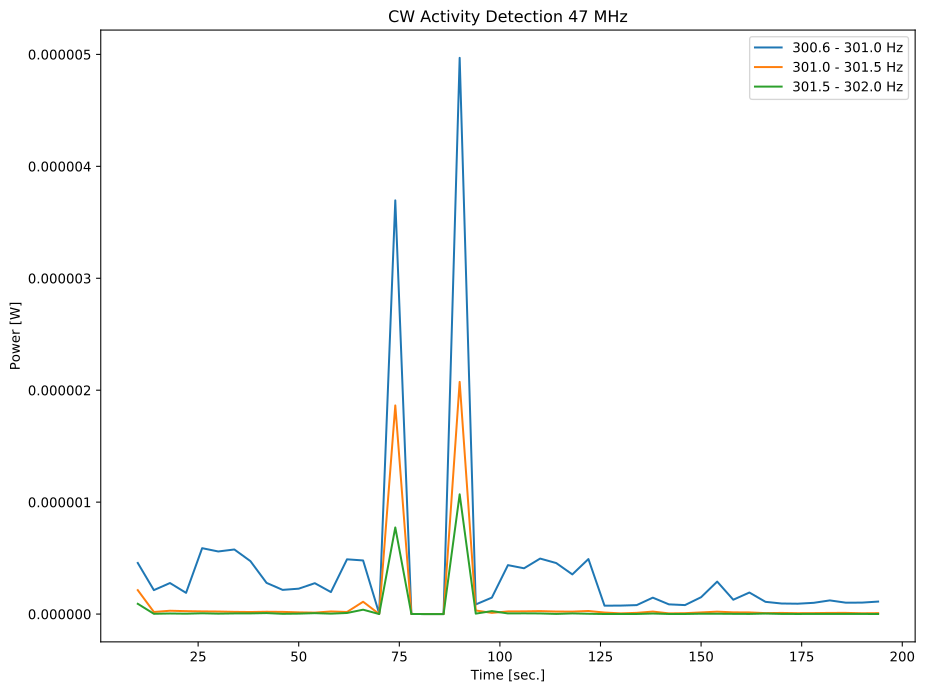
Activity detection vs. time with CW radar at 47 MHz.
The subspace estimator outputs two vectors.
The first vector is the frequency estimate and the second vector is the corresponding singular value.
The larger the singular value, the higher the confidence in the frequency estimate.
This can be used as a qualifier to discard unlikely targets.
Also, targets outside a plausible Doppler shift (or range, for FMCW) can be discarded by inspection.
During daylight hours (and other more occasional events) D-region absorption increases immensely for VLF, LF, MW, and lower HF frequencies.
The frequency of interest passing through the D-region is very important; the daytime D-region attenuation is hundreds of dB [1].
[1] Sir Edward Appleton, W.R. Piggott, Ionospheric absorption measurements during a sunspot cycle, J. Atm. Terr. Phys., (5)1, 1954, 141-172, https://dx.doi.org/10.1016/0021-9169(54)90029-X.
Abraham, Saji, et al. “Ionospheric absorption on October 24, 1995 solar eclipse.” Geophysical research letters 25.15 (1998): 2945-2947. https://doi.org/10.1029/98GL01781
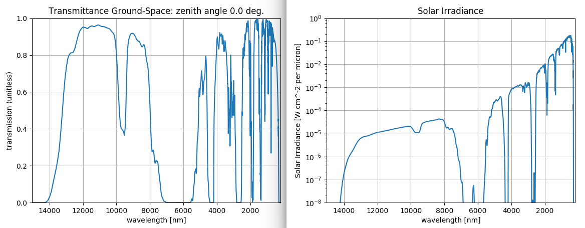
SolarIrradiance.py
is a LOWTRAN model accessed through Python of Solar Irradiance, as well as transmittance ground-space.
Lowtran solar irradiance model and transmittance.
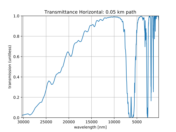
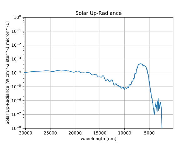
Also added was the user data mode, where your own measured temperature, pressure, humidity, etc. can be used to compute the transmittance spectrum more accurately.
Lowtran transmittance using user-provided data for model inputs.
Lowtran solar up-radiance using user-provided data for model inputs.
A
radar based on Red Pitaya
may operate for calibration or even primary purposes on lowband VHF (25-50 MHz).
A primary reason one might use a radar on lowband VHF is for example measuring human, animal or vehicle targets using
global license-free frequency bands.
Such a radar can be handheld and battery powered, with collapsible antenna rods.
The humanitarian demand for a such a radar could be significant as a much more compact and economical radar than the
coffee can radars
that have become popular after I developed the first such “personal radar” in 2006.
There are global license-free frequencies in the 40-50 MHz range.
One can consider the
US license-free frequencies in the 40-50 MHz range.
For signal processing, using FFT-based methods breaks down for the narrowband radar because the frequency separation is too small.
A common PC runs out of RAM, and certainly a small embedded CPU would as well.
I tried to squeeze more frequency resolution out of the FFT, but a normal 8 GB laptop would run out of RAM, so it’s not workable on a 1 GB RAM Raspberry Pi 3.
By instead using subspace estimation methods to find beat frequency
CWsubspace.py
the narrowband, small beat frequency separation seems initially possible in simulation.
In initial measured data, the clipped ADC due to building 60 Hz pickup makes lots of extra fake beat frequencies.
While working on the hardware fix to the clipped ADC (1:9 or 1:16 transformer for Red Pitaya input), one can make use of existing slightly clipping data by implementing a digital bandpass filter around the known center frequency.
This is “fair” and standard practice, even without the clipping.
Signal subspace estimation techniques like ESPRIT and RootMUSIC find applications in radar, whether angle of arrival estimation or for close-spaced noisy sinusoid frequency estimation.
There are
bounds on subspace estimation performance
as with any signal estimation technique, but in a subset of cases involving short range, narrowband radar, subspace estimators may have significant advantages.
Subspace estimators give excellent performance vs. FFT for a given SNR, particularly with low SNR, with far lower RAM demands for a given accuracy vs. FFT.
Mitigate CPU usage by using optimized
signal subspace estimation FORTRAN code.
Use a priori on number of sinusoids stronger than desired signal expected.
Filter signal before estimation necessary as with FFT to constrain estimate to expected frequency range (e.g. automobiles not expected to drive 500 m/s)
To parallelize the work of modeling and designing analysis, we can model expected beat frequencies for CW and/or FMCW.
Simulate estimation with noisy sinusoids at the modeled beat frequencies.
CW only gives Doppler.
A model for beat frequency vs radial velocity is is
piradar/CW_doppler.py
as
discussed here:
fbeat = 2 * v * ftx/(c-v)
FMCW can give range and velocity via the FMCW beat frequency.
FMCW typically linearly sweeps the transmit frequency.
Non-linearities in the sweep broaden the target uncertainty (increase error).
A model for expected beat frequencies is in
CalcBeat.py.
FMCW beat frequencies in Hertz are defined by
f_beat= R * B/(T c)
where R is one-way range to target [meters], c is speed of light, T is chirp cadence [Hz].
B = f_max - f_min
chirp RF bandwidth
./CalcBeat.py -tm .1 -b 10e6
For point target ranges [1, 10, 50] meters you may expect beat tones [‘0.7’, ‘6.7’, ‘33.4’] Hz.
Using 10.0 MHz RF bandwidth, you may expect 15 meters range resolution by:
ΔR = c/(2 B)
If you sweep from 902..928 MHz, then B=26 MHz.
However, using a priori knowledge about the targets, super-resolution techniques can enable better resolution proportional to SNR.
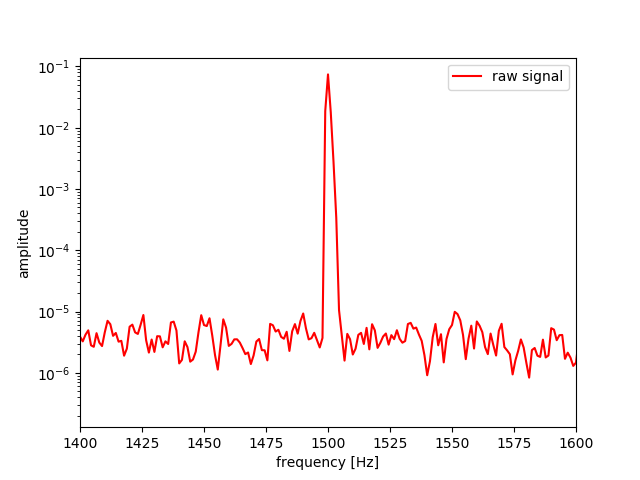
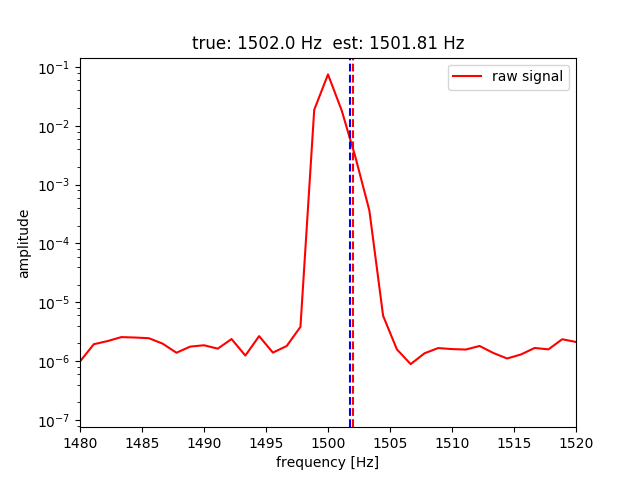
These plots demonstrate a system (CW or FMCW) that results in a true fbeat = 2.0 Hz.
The estimation is performed by ESPRIT in piradar/CWsubspace.py
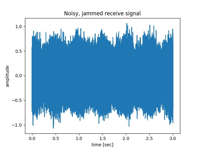
Noisy time domain received signal from CW radar. Dominant signal is carrier leakage as expected for non-nulled CW radar.
Frequency domain: receive signal is blurred together with CW carrier leakage--actual separation 2 Hz. FFT exhausts PC RAM without giving enough separation to resolve target beat frequency.
Frequency domain: receive signal is blurred together with CW carrier leakage--actual separation 2 Hz. Estimation error ~ 10%.
Estimation error with ESPRIT and block length 1000 gave beat frequency estimation error of order 10%.
This simulation from
piradar/FMCW_sim.grc
was conducted with GNU Radio and the standard built-in modules.
The parameters were chosen for convenience of display in plots, not for a particular scenario.
Parameter
Value
Units
sample rate
1e6
samples/sec
sweep freq
50
Hz
VCO modulation
ramp (sawtooth)
sweep bandwidth
100e3
Hz
The simulation was performed at baseband, so upon using DUC & DDC one could sweep from 40.7 to 40.8 MHz or whatever desired frequency.
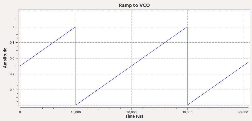
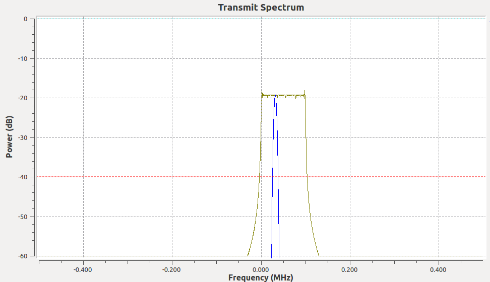
FMCW 50 Hz ramp input voltage to VCO.
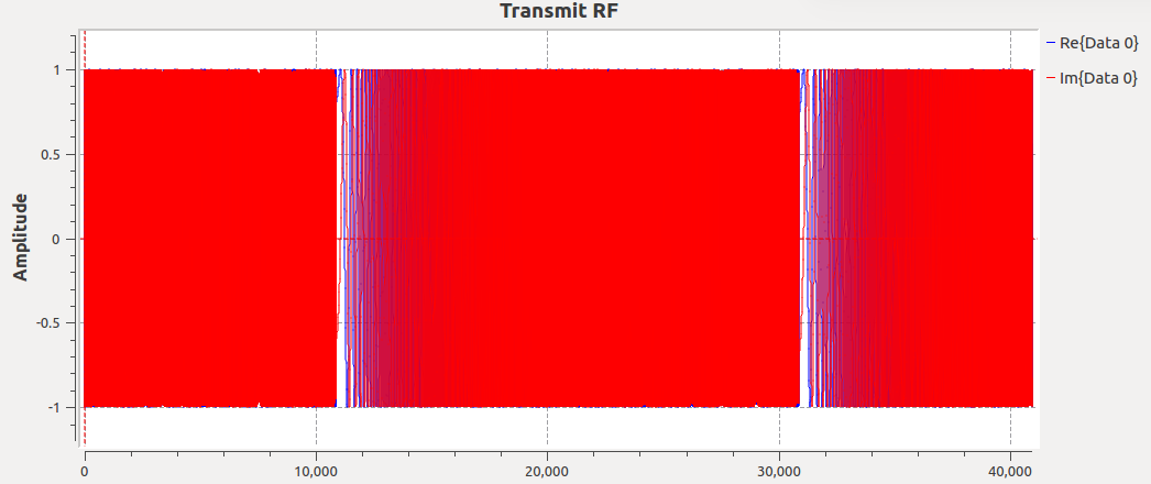
VCO output in time domain. Sweep starts at 0 Hz and goes to 100 kHz in baseband at 1 MHz sampling rate with 50 Hz cadence.
VCO output in frequency domain. Sweep starts at 0 Hz and goes to 100 kHz in baseband at 1 MHz sampling rate with 50 Hz cadence.
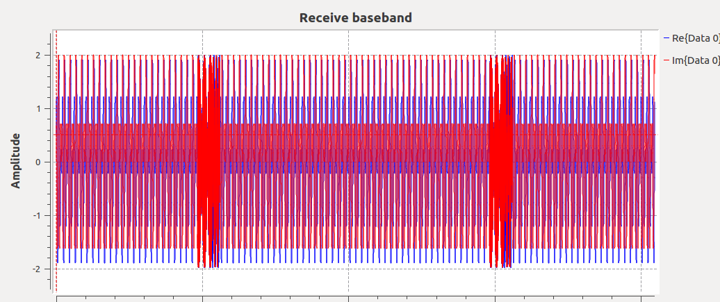
FMCW Demodulated output--pair of targets. Periodic glitches due to discontinuity at ramp reset.
The glitches are customarily eliminated in a straightforward way by dropping those samples (or skipping them) since they are inherently periodic.
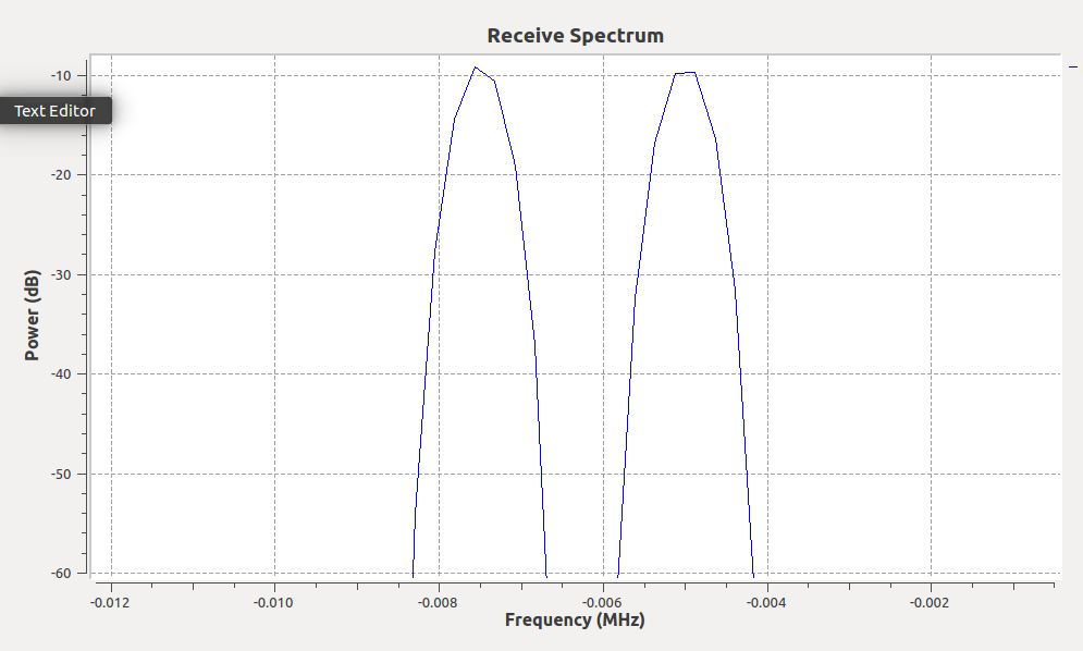
FMCW Demodulated output spectrum--pair of targets. Periodic glitches due to discontinuity at ramp reset.
The receive spectrum shows two distinct targets–one with a beat frequency of about 7 kHz and another at about 4.7 kHz.
This corresponds to a range of about 210 km and 140 km – perhaps an F-region and E-region ionosphere radar return, respectively.
The parameters used in these plots were more suitable for HF (2-10 MHz) measurements of the ionosphere.
Using low-band VHF, we can sweep a few MHz in the license-free bands, and sweep at a faster cadence.
Let’s say the radar sweeps 5 MHz at a 1 kHz cadence, then a target 20 meters away returns a 667 Hz beat frequency.
When developing an embedded sensing system, one of the very first steps is making a method to retrieve raw data from the sensor and store it.
Prevention of later problems due to unforeseen data acquisition issue scan be easily obtained by obtaining and retaining the raw data stream an essential specification from day one.
This raw data stream is the basis for important registration and unit tests.
With experience and a forward model of what to expect, one quickly gains deep insight into what is always at least partially the black box of the embedded system.
Some of the factors thereby determined include
Sample rate verification: too fast or slow?
interference: bad grounds, environmental
signal dropouts: system can’t keep up with data rate, race conditions
unexpected signals (good or bad) mixing with desired signal
Based on the above:
Is analog and or digital filter needed?
Is a PCB or circuit redesign needed
Is more advanced signal processing or different embedded CPU or GPU needed?